Anomaly Detection with SDR Data

Software-Defined Radio (SDR) technology has revolutionized how we interact with radio frequency (RF) signals. With the ability to capture and analyze vast amounts of RF data, SDR systems create new opportunities for detecting anomalous signals in real-time. In this post, we'll explore building an anomaly detection system for SDR data using statistical analysis of time-frequency domain characteristics.

Our approach will move beyond simple threshold-based detection methods to identify subtle anomalies that may indicate interference, unauthorized transmissions, or equipment malfunctions. By analyzing multiple statistical moments across different frequency bands, we can build a robust detection system that adapts to varying signal environments.

We're working with data collected from an Ettus Research USRP B200-mini device, which provides I/Q (In-phase and Quadrature) samples representing complex radio signals. Let's first look at our dataset:

• Sample rate: 40 MHz
• Center frequency: 935 MHz
• Format: Complex 32-bit floating point (cf32_le)
• Duration: ~0.6 seconds (24 million samples)

The data is stored in SigMF format (Signal Metadata Format), which pairs raw binary samples with JSON metadata that describes the signal characteristics.

{
    "captures": [
        {
            "capture_details:gain": 0.0,
            "core:datetime": "2024-08-12T12:59:25Z",
            "core:frequency": 935000000.0,
            "core:global_index": 0,
            "core:sample_start": 0
        }
    ],
    "global": {
        "core:datatype": "cf32_le",
        "core:description": "VL SigMF recording",
        "core:extensions": [
            {
                "name": "antenna",
                "optional": true,
                "version": "1.0.0"
            },
            ...
        ],
        "core:hw": "SDR 0 Ettus Research LLC USRP B200-mini",
        "core:recorder": "VL Sensor v3.2.0",
        "core:sample_rate": 40000000.0,
        "core:version": "1.2.2"
    }
}

Before building our detection algorithm, we need to understand the characteristics of our signal data. Let's examine various visualizations and statistical properties to identify patterns and potential anomalies.

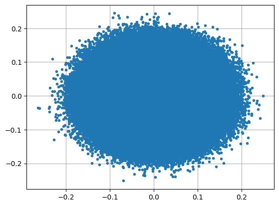
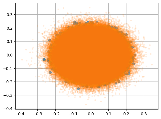
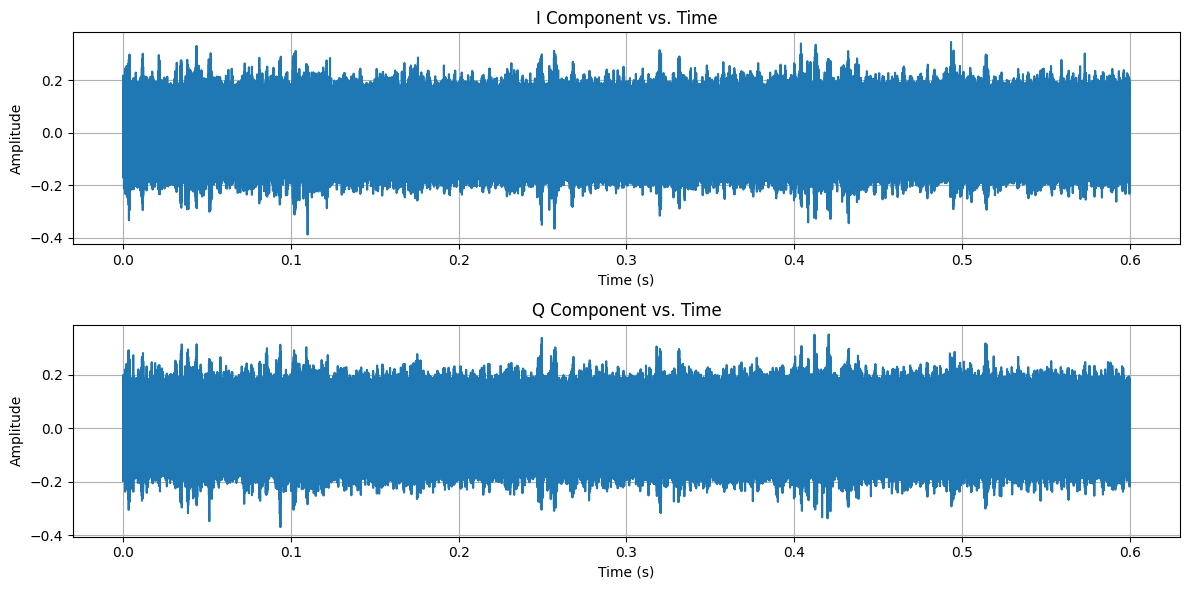
Time Domain Analysis

Looking at the I and Q components over time reveals interesting patterns:

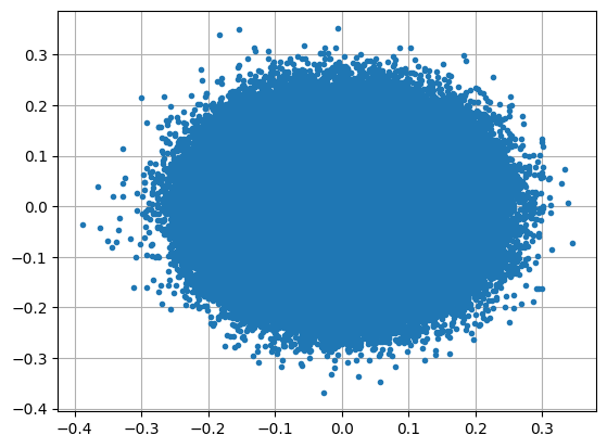
Key observations:

• Similar patterns in both I and Q components
• No major signal dropouts
• Stable baseline with occasional power spikes
• Multiple noise sources and ambient signals

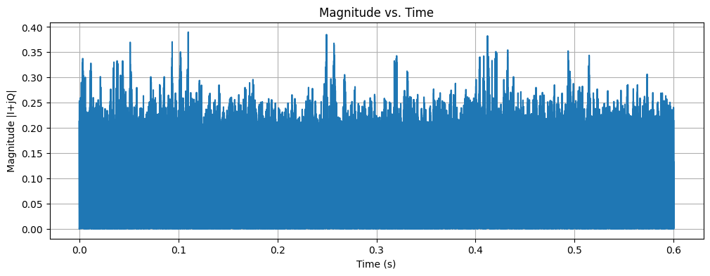
Signal Magnitude

The signal magnitude (|I+jQ|) provides a clearer view of power variations over time:

This confirms a stable envelope carrier around 0.2 with multiple irregular spikes.

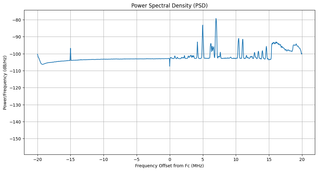
Frequency Domain Analysis

The power spectral density (PSD) reveals the frequency composition of our signal:

The PSD shows multiple discrete frequency components with varying power levels. Note the interesting behavior between 15-20 MHz offset, which shows a raised noise floor.

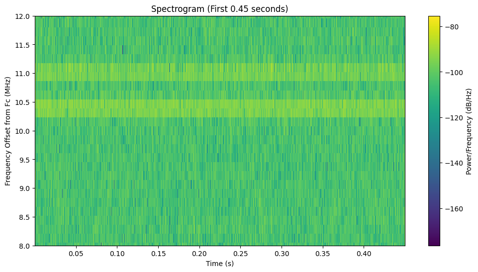
Time-Frequency Analysis

A spectrogram gives us both time and frequency information simultaneously:

The spectrogram reveals:

• Stable horizontal lines indicating consistent narrowband signals
• Possible vertical bands showing power fluctuations over time
• No obvious frequency hopping or chirp patterns

To capture the complex behavior of our signals, we'll analyze three key statistical moments across different frequency bands:

1. Mean Power

The average power in each frequency band helps us identify strong carriers and distinguish them from noise. Significant changes in mean power can indicate new signals appearing or existing signals disappearing.

2. Kurtosis

Kurtosis measures the "tailedness" of a distribution - how much the distribution is driven by outliers. High kurtosis in our signal power indicates intermittent or bursty behavior, while low kurtosis suggests more consistent power levels.

Our data shows interesting kurtosis peaks at specific frequency offsets (e.g., around 5 MHz and in the 15-20 MHz region), highlighting frequencies with highly non-Gaussian behavior.

3. Skewness

Skewness indicates the asymmetry of a distribution. Positive skewness in our power values suggests occasional power bursts above the baseline, while negative skewness would indicate power dropouts.

Examining the skewness at -15.5 MHz confirms our kurtosis finding, showing a highly right-skewed distribution of power values with occasional high-power events.

Based on our exploratory data analysis, we'll implement a multi-band statistical anomaly detection system. Our approach:

1. Define Frequency Bands of Interest: Based on our EDA, we'll monitor multiple frequency bands, including the strong carriers at +7 MHz and +10 MHz, as well as potentially anomalous regions.
2. Calculate Statistical Baselines: For each band, we'll establish baseline values for mean power, kurtosis, and skewness from our training data.
3. Apply Z-score Thresholding: We'll detect anomalies by looking for statistical moments that deviate significantly (e.g., Z-score > 3.5) from the baseline.
4. Time-Block Processing: Process incoming signals in overlapping time blocks to enable near real-time detection.

Here's a simplified implementation of our approach:

import numpy as np
import scipy.signal as signal
import scipy.stats as stats

# Define frequency bands of interest (in Hz offset from center frequency)
FREQ_BANDS_HZ = {
    'LowNeg': (-16e6, -15e6),
    'Quiet1': (-10e6, 0.0),
    'Intermittent3MHz': (2.8e6, 3.2e6),
    'Carrier7MHz': (6.8e6, 7.2e6),
    'Carrier10MHz': (9.8e6, 10.8e6),
    'Broadband15_20MHz': (15e6, 19.8e6),
}

# Configure detection parameters
BLOCK_SIZE_SEC = 0.1    # Analysis block size in seconds
OVERLAP_RATIO = 0.5     # Overlap between consecutive blocks
Z_THRESHOLD = 3.5       # Z-score threshold for anomaly detection

# Define function to calculate statistics for each frequency band
def calculate_block_statistics(block_data, fs, freq_bands_hz):
    stats_dict = {band_name: {} for band_name in freq_bands_hz}
    
    # Calculate spectrogram
    f_spec, t_spec, Sxx = signal.spectrogram(
        block_data, fs=fs, 
        nperseg=256, noverlap=128,
        return_onesided=False, scaling='density'
    )
    f_spec = np.fft.fftshift(f_spec)
    Sxx = np.fft.fftshift(Sxx, axes=0)
    
    # Calculate stats per frequency bin across time
    P_all_bins = np.mean(Sxx, axis=1)          # Mean power
    K_all_bins = stats.kurtosis(Sxx, axis=1)   # Kurtosis 
    S_all_bins = stats.skew(Sxx, axis=1)       # Skewness
    
    # Aggregate stats over defined bands
    for band_name, (f_low, f_high) in freq_bands_hz.items():
        band_indices = np.where((f_spec >= f_low) & (f_spec <= f_high))[0]
        
        if len(band_indices) > 0:
            stats_dict[band_name]['Power'] = np.mean(P_all_bins[band_indices])
            stats_dict[band_name]['Kurtosis'] = np.nanmean(K_all_bins[band_indices])
            stats_dict[band_name]['Skewness'] = np.nanmean(S_all_bins[band_indices])
            
    return stats_dict

# Baseline calculation and anomaly detection shown in the next section...

Let's examine the performance of our anomaly detection system using a separate test dataset:

Our system successfully detected multiple anomalies across different frequency bands:

• Significant power variations in the Carrier7MHz band (Z-score &gt 5)
• Unusual kurtosis in the Broadband15_20MHz region (Z-score &gt 10)
• Abnormal skewness in the LowNeg band (Z-score &gt 15)

The system processes data in near real-time, with each 0.1-second block being analyzed in approximately 0.15 seconds on standard hardware. Using overlapping blocks helps ensure we don't miss transient anomalies.

We've demonstrated a powerful approach to anomaly detection in SDR data using statistical moments in the time-frequency domain. By analyzing mean power, kurtosis, and skewness across multiple frequency bands, we can detect subtle anomalies that might be missed by simpler methods.

This approach could be extended in several ways:

• Machine Learning Integration: Replace static Z-score thresholds with ML models trained to recognize complex patterns
• Adaptive Baseline: Implement sliding windows for baseline calculations to adapt to slowly changing environments
• Feature Engineering: Add additional statistical features like spectral flatness, entropy, or autocorrelation
• Classification: Move beyond binary anomaly detection to classify different types of signal anomalies

SDR-based anomaly detection has applications across many domains, including spectrum monitoring, interference detection, cognitive radio, and security applications. As SDR hardware becomes more accessible, these techniques will play an increasingly important role in managing our shared RF spectrum.